Engineering a Unified AI Storage Layer with JuiceFS, TiKV, and Ceph

index

When a training worker waits for its next batch, the delay may be in a directory lookup, a cold data block, or an overloaded filesystem client. From the application’s perspective, each can look like idle compute. Each needs a different fix.

A shared AI storage platform has to make those dependencies manageable across very different workloads. Training workers read samples, Spark executors discover partitions, model servers load weights, and backup jobs walk the namespace. They can share data while making different demands on naming, consistency, latency, and durability.

JuiceFS, TiKV, and Ceph offer a clean separation of responsibilities: filesystem semantics at the client, transactional metadata in TiKV, and payload objects in Ceph RADOS. The central engineering question is what must happen between an application asking for data and being able to trust the result. That question connects the read path, checkpoint durability, cache placement, and recovery.

Tuhu’s deployment, described by Haitang Yang, provides a concrete example: more than 100 million files, a five-node TiKV cluster, and consolidation across training, inference, ClickHouse, and backups, with NFS, Alluxio, MinIO, and SeaweedFS retired in stages. Its architecture and reported results anchor the analysis that follows.

Start with the boundaries between components

A file has two kinds of state: the metadata that identifies and describes it, and the bytes that make up its contents. JuiceFS connects the two. TiKV stores the namespace and data mappings; Ceph stores the objects those mappings reference.

Component	Responsibility	Useful diagnostic question
JuiceFS clients	Translate file operations into metadata and block operations	Is time spent resolving names, buffering, or fetching blocks?
TiKV	Persist the namespace and file-to-data mappings transactionally	Are metadata transactions delayed or contending?
Ceph RADOS	Place objects and maintain their configured redundancy	Are OSD queues, media, or recovery consuming the budget?
Local data cache	Reuse previously fetched blocks	Is this node reading a warm working set?
Application KV cache	Reuse model attention state	Is this state compatible with the request and cheaper to load than recompute?

This split makes a slow open() a different investigation from a slow bulk read(). It also creates a recovery obligation: preserving the objects is insufficient if the namespace that locates them is lost.

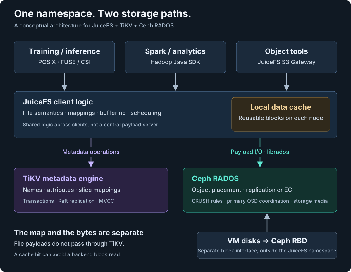
JuiceFS clients split operations into a TiKV metadata path and a librados payload path to Ceph. Local cache is a client concern; RBD exposes a separate block interface. — Figure 1 — Separate metadata and payload paths. The client box groups logic used across access methods; it does not represent a central server.

One namespace, several entry points

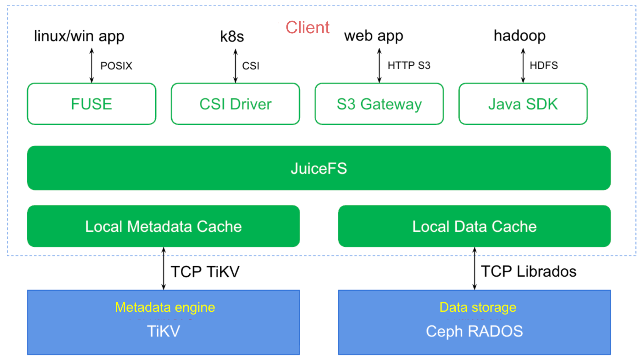
For a Python training process, a FUSE mount presents file operations through the operating system. In Kubernetes, CSI manages volume provisioning and the mount lifecycle. The mounted client handles subsequent reads and writes; CSI does not add another payload hop to every operation.

The JuiceFS Hadoop Java SDK integrates with Hadoop’s filesystem interface, allowing Spark and related tools to use JuiceFS without routing every operation through a FUSE mount. That changes the integration path, while retaining the same filesystem metadata and backing data.

For object-oriented applications, the JuiceFS S3 Gateway exposes the filesystem through an S3-compatible API. This gateway sits above JuiceFS. It is distinct from configuring JuiceFS to store its internal blocks through an S3 backend such as MinIO or Ceph RGW.

The distinction matters operationally. Internal objects are pieces of the filesystem’s representation; paths, file lengths, and block mappings live in the metadata layer. Pointing an S3 client at the backing store exposes that representation, not the application’s file listing.

Shared storage still needs a shared publication convention. An ingestion service and a trainer must agree on when a dataset is ready, even if one writes through S3 and the other reads through a mounted path. Validate the operations that establish that agreement: rename, permissions, object metadata, multipart uploads, and visibility to concurrent readers.

RBD remains a separate interface

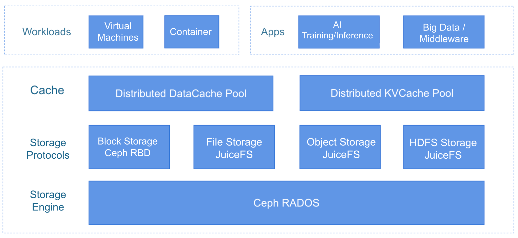
Ceph RBD supplies virtual block devices for VM disks. Those devices can share a Ceph cluster with JuiceFS, but they do not become files in the JuiceFS namespace simply by using the same cluster. Similarly, JuiceFS over RADOS is not JuiceFS layered over CephFS: this design supplies filesystem metadata through TiKV, without inserting a CephFS metadata server. See Ceph’s architecture overview.

Figures 2–3: Tuhu's platform and deployment architecture

Tuhu's original platform diagram showing workloads, DataCache and KVCache pools, storage interfaces, and underlying storage engines. — Figure 2 — Tuhu's unified storage platform. Credit: Haitang Yang / Tuhu, via JuiceFS.

Tuhu's original JuiceFS deployment diagram with separate metadata and Ceph RADOS data connections. — Figure 3 — JuiceFS deployment at Tuhu. Credit: Haitang Yang / Tuhu, via JuiceFS.

Follow a read from pathname to payload

Consider a training worker reading 256 KiB starting 8 MiB into /datasets/run-42/shard.bin.

JuiceFS must resolve the path, identify the file, map the requested range to stored data, and return the bytes in file order. Cached directory entries and attributes can satisfy some of those steps locally. The dependencies remain even when the network round trips disappear.

The documented internal representation has three relevant units:

A chunk is a 64 MiB logical region of a file.
A slice describes data written within a chunk. Overlapping writes can leave multiple slices contributing to the current view.
A block is an object-storage and local-cache unit, with a default maximum size of 4 MiB.

Chunk boundaries organize lookup; they do not force every small file to occupy 64 MiB. Likewise, the 4 MiB block size does not imply that a ten-byte file requires a four-megabyte payload object.

For file offset $o$ and logical chunk size $C$ :

\text{chunk index} = \left\lfloor \frac{o}{C} \right\rfloor, \qquad \text{offset within chunk} = o \bmod C.

Our request falls in chunk 0, at an offset of 8 MiB within that chunk. The client still needs the slice mappings to locate its bytes. Previous writes may have replaced part of the range, so dividing the offset by the block size cannot, by itself, produce the right object key.

The following is explanatory pseudocode, not a JuiceFS API:

def read_file_range(path, offset, length):
    inode = namespace.resolve(path)             # metadata/cache
    extents = namespace.map_range(inode, offset, length)
    output = bytearray(length)
 
    for extent in extents:
        if extent.is_hole:
            continue                           # output is already zeroed
        block = local_cache.get(extent.block_id)
        if block is None:
            block = object_store.read(extent.block_id)
            local_cache.put(extent.block_id, block)
        copy_requested_bytes(block, extent, output)
 
    return output

Real clients add parallelism, buffering, readahead, retries, and consistency rules. The architectural point is that payload bytes do not transit TiKV. Once mappings are available, block reads proceed against the local cache or object store, as described in the I/O processing documentation.

Profile those paths separately. Scanning a directory containing millions of entries can make dataset startup expensive even when sequential reads are fast. Loading a cold model can spend most of its time transferring tens of gigabytes after path resolution has already finished. Increasing backend bandwidth helps only the part of the job waiting on that bandwidth.

Follow a write to its durability boundary

A read must find the right bytes. A write must also define when those bytes are safe to rely on. A successful write() can mean that a buffer accepted data while remote storage is still catching up.

In JuiceFS’s default mode, buffered payloads are uploaded before the associated file-write metadata is committed. fsync() and close() can force upload. The optional client --writeback mode instead stages data locally, commits metadata, and uploads asynchronously. This ordering is documented in the client write-cache guide.

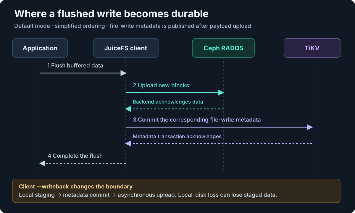
Default JuiceFS flush uploads new blocks to RADOS, receives a data acknowledgement, commits the file-write metadata to TiKV, and completes the flush. Client writeback stages locally before asynchronous upload. — Figure 4 — Ordering at the flush boundary. The final acknowledgement is distinct from an ordinary buffered write returning. Earlier namespace operations, retries, and backend replication messages are omitted.

Consider a failure between the two stores. If payload upload succeeds but publication of its mapping fails, an object can remain without a live file reference. Reversing the order would create a more dangerous possibility: a reader discovers a mapping whose payload is unavailable. The filesystem has to manage these intermediate states because no single transaction spans TiKV and every Ceph OSD.

Client writeback deliberately changes that boundary. During the staging window, losing the local disk can lose newly acknowledged file data. It may suit regenerable intermediate data, but it should not silently become the checkpoint durability policy.

This distinction belongs in every write benchmark. Timing writes into memory, local staging, and a flush to redundant remote storage measures three different completion conditions. Throughput is meaningful only alongside the condition that ends the timer.

For a checkpoint, make publication an explicit sequence: write a versioned artifact, flush it and check errors, then publish a manifest or readiness marker that readers understand. Test the required rename and crash-recovery behavior on the deployed client version. The application needs a clear point at which a partially written checkpoint becomes a usable one.

Scale the namespace by workload, not file count

TiKV makes the namespace a distributed database workload. Its JuiceFS integration guidance describes Raft replication, multiversion concurrency control, and garbage collection of obsolete versions.

Transactions keep related namespace facts in agreement. Moving a name between directories, for example, requires coordinated changes to the relevant records. Readers must observe a valid filesystem state while those changes happen.

Tuhu’s five-node deployment describes the cluster’s size, not the replica count of every metadata partition. To reason about availability and latency, inspect replication policy, placement, quorum health, and transaction contention separately.

The workload shape matters as much as cardinality. Compare two hypothetical jobs:

Workers independently read immutable files distributed across many directories.
Thousands of workers repeatedly create and rename files beneath one shared directory.

The same number of files can produce very different contention. In the second workload, an extra data disk cannot remove serialization on hot metadata records.

Track operation latency by type, transaction retries, compaction pressure, and hot paths. Include garbage collection in that view: retained MVCC versions consume resources even after the current namespace looks stable. A file count describes how much state exists; these measurements describe the work required to maintain it.

Strong metadata storage alone does not promise that every client cache is instantly refreshed. Applications must still observe the filesystem’s documented cross-client visibility rules. An immutable dataset plus a deliberate publication step is much easier to reason about than many writers modifying files that training workers already have open.

Native RADOS shortens one part of the path

Once the client has resolved the data mapping, the backend interface determines how its object request reaches Ceph. JuiceFS can take either of two paths:

S3 backend:
JuiceFS → S3/HTTP → Ceph RGW → RADOS
 
Native backend:
JuiceFS → librados → RADOS

The native path removes the S3 gateway, while bringing a Ceph-enabled JuiceFS build, compatible librados, and Ceph configuration into the client deployment. In Kubernetes, those dependencies belong in the Mount Pod’s image and configuration, as specified in the RADOS integration documentation.

Ceph’s monitors provide cluster-map information; OSDs serve objects. Placement and redundancy remain Ceph’s job. Removing RGW does not remove the primary OSD’s coordination, network traffic, checksumming, device latency, or erasure-coding work.

To locate the benefit, break an operation into an approximate latency budget:

T_{\text{operation}} \approx T_{\text{namespace}} + T_{\text{client}} + T_{\text{transport}} + T_{\text{backend}} + T_{\text{queue}}.

Some work overlaps, so the expression is a profiling aid. Removing a forwarding layer can matter more for a tiny request than for a long sequential transfer because fixed overhead occupies a larger fraction of the operation.

The next bottleneck still matters. An overloaded metadata database or a saturated device can dominate the budget after the gateway is gone. This also sets a limit on the benchmark interpretation later: comparing MinIO with Ceph changes the backend as well as the protocol path. It cannot isolate the cost of RGW.

Erasure coding changes the economics of object size

For an erasure code with $k$ data shards and $m$ parity shards, the ideal large-object storage factor is:

A_{\text{ideal}} = \frac{k+m}{k}.

A 6+3 profile approaches 1.5 physical bytes per logical byte for sufficiently large objects, before other overhead. Three-way replication requires three copies. For small objects, however, allocation granularity can overwhelm that theoretical saving.

Work through the allocation floor

Assume a simplified layout with a 4 KiB allocation unit and nine allocated shards. A ten-byte payload can occupy:

9 \times 4\ \text{KiB} = 36\ \text{KiB}, \qquad A_{\text{space}} = \frac{36\times1024}{10} \approx 3686.

If the layout avoids allocating unused data shards and needs one data allocation plus three parity allocations, the same illustrative accounting becomes:

(1+3)\times4\ \text{KiB}=16\ \text{KiB}.

The modeled footprint falls by about 55.6%, yet remains large relative to ten useful bytes. Object metadata, database structures, fragmentation, and recovery reserves would add further costs. Capacity planning therefore needs an object-size distribution, not just a total byte count.

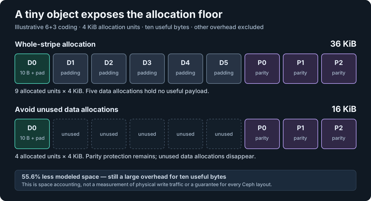
Illustrative 6 plus 3 erasure-coded allocation for a ten-byte object: six data and three parity allocations occupy 36 KiB; avoiding unused data allocations reduces that to one data and three parity allocations, or 16 KiB. — Figure 5 — Illustrative allocation model for a ten-byte payload: 6+3 coding with 4 KiB allocation units. Actual footprints depend on pool and device configuration. The comparison measures space, not write bandwidth.

Space amplification and write amplification are different measurements. Space amplification compares resident physical bytes with logical bytes. Write amplification compares bytes written at a chosen lower layer with application bytes written. Reducing padding can improve both, but a disk-usage comparison does not measure the second one.

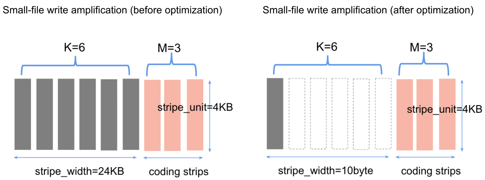
Ceph’s Fast EC engineering article describes three separate mechanisms: avoiding whole-stripe padding for small objects, reading only needed portions, and reducing work for partial writes. Parity-delta writes update parity from changed data rather than always rebuilding the entire stripe; the implementation selects an appropriate write strategy.

The file-to-object mapping is crucial here. JuiceFS represents file edits using new immutable blocks, so a 4 KiB file overwrite does not necessarily become a 4 KiB overwrite of the same RADOS object. Before attributing a gain to parity-delta writes, inspect the object operations the client actually emits. An optimization matters only if the workload reaches the path it optimizes.

The Ceph optimization documentation ties allow_ec_optimizations to Tentacle or later, with monitor/OSD and coding-plugin requirements. Enabling it changes the stored representation and cannot be reversed by simply clearing the flag. Treat pool layout and stripe-unit selection as deployment design decisions, backed by tests on the actual release.

An EC profile also needs a failure-domain policy. CRUSH placement determines whether a host failure removes one shard or several. Recovery consumes spare capacity and bandwidth while applications are still doing work. Evaluate the pool under those degraded conditions, following the placement constraints in Ceph’s erasure-code operations guide.

Figure 6: the deployment's allocation comparison

Original before-and-after illustration accompanying the case study's small-object erasure-coding optimization. — Figure 6 — Small-object allocation before and after optimization. Credit: Haitang Yang / Tuhu, via JuiceFS.

Put cached data where the work will run

Once the object path is efficient, avoiding repeated transfers becomes the next opportunity. For a simple training workload, let clients request $D$ bytes per epoch with an aggregate byte-weighted cache hit ratio of $h$ . Backend bytes needed to satisfy those demand reads are approximately:

B_{\text{backend}} \approx D(1-h).

This counts the requested bytes that miss the cache. Prefetch over-read, retries, and backend redundancy add traffic beyond the model. The implication is a scheduling constraint: a cache warm on worker A does not make worker B warm. Reshuffling work can turn yesterday’s cache hits into today’s backend reads.

The JuiceFS cache guide distinguishes kernel caching, client buffering, and local data caching. Calling all of these “the cache” hides which layer a measurement exercised. A small object can hit locally while its metadata still needs validation; a sequential reader can fetch data it never consumes if readahead is poorly matched.

KV reuse has to beat recomputation

LLM KV caching adds a different identity problem. Cached keys and values depend on the model, the exact preceding token context, and representation details. A filename alone cannot establish whether state is reusable. The serving integration must define compatible cache keys, ownership, eviction, and transfers.

For a candidate offload, compare the cost of restoring state with the cost of recomputing it:

T_{\text{restore}} \approx T_{\text{lookup}}+ \frac{S_{\text{KV}}}{B_{\text{effective}}}+T_{\text{movement}}.

The final term covers host/device movement and conversion not already included in the effective transfer bandwidth. The total, including queueing, must fit the request’s latency budget and improve on recomputation.

For example, transferring a hypothetical 2 GiB cache over an effective 4 GiB/s path already takes 0.5 seconds before additional overhead. That might be attractive for a long expensive prefix and unacceptable for a short interactive request. A storage throughput number cannot answer the serving question by itself.

Tuhu describes DataCache and KVCache layers. Its proposed HBM → DRAM → local SSD → shared-storage KV hierarchy remains a roadmap item, alongside hybrid-cloud management, broader lakehouse integration, and private-Ceph tiering. The architecture supports discussing those possibilities; the account does not establish a completed four-tier serving implementation.

A prototype should establish which requests reuse state, where that state sits when scheduling occurs, and whether retrieval improves time to first token under contention. Storage provides the capacity to retain state. Scheduling and transfer costs determine whether retaining it helps.

The mount process is part of the reliability boundary

Every path above depends on a live userspace client. If the Mount Pod runs out of memory, applications can lose access even while TiKV and Ceph remain healthy. Client resource management is therefore part of storage availability.

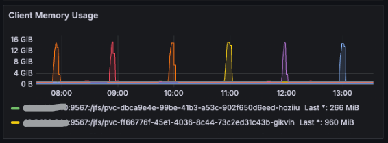
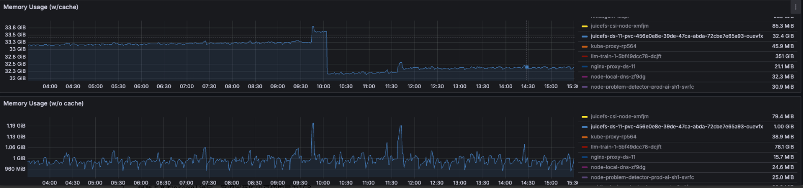
Tuhu reports two OOM patterns involving metadata-backup work and page-cache growth. Its remedies include dedicated backup jobs, adjusted memory limits, isolated cache directories, and bounded local cache capacity. Both incidents show how work near the data path can destabilize the process serving it.

Give backups an explicit owner

The reported backup failure involved a large metadata export hitting a RADOS object-size limit, followed by repeated failures and memory growth. A backup uploaded directly to the backend need not follow the block-splitting path used for ordinary files. That explains why an object-size limit can matter even when the filesystem handles much larger files. Ceph exposes the configurable osd_max_object_size; its Squid reference lists a 128 MiB default. Investigate the exporter’s behavior before changing that limit.

At large namespace sizes, metadata export is a meaningful workload. Schedule it with its own resource budget, retry policy, destination-size checks, and monitoring. Moving export into a dedicated job should preserve backup coverage rather than merely remove work from application mounts.

The metadata-backup documentation also contains a correctness constraint: juicefs dump is not a point-in-time snapshot while writes continue. Binary export is available in newer clients and has different resource characteristics. A recovery plan must be matched to the deployed version and the application’s consistency needs.

Backing up metadata alone is also insufficient. Recovery needs the data objects referenced by the restored namespace. Retention and deletion policies therefore have to preserve a compatible recovery point across both stores.

Validate recovery by restoring into an isolated environment, resolving a representative manifest, reading its files, and checking their contents against known expectations. The acceptance condition is a usable dataset restored within the recovery target. A successful export is only one step toward that result.

Diagnose memory at the cgroup boundary

Process RSS, container memory, and a dashboard’s working-set metric are different views. File-backed cache can contribute to memory pressure even when the client’s application heap looks modest.

Start with the enforcement mechanism. On Linux, cgroups enforce container memory limits; kernel reclaim and allocation failure determine cgroup OOM behavior. A dashboard’s working_set_bytes reports a view of usage, rather than controlling that decision. Kubelet eviction under node pressure is a separate mechanism. The distinction is documented in Kubernetes resource management and the cgroup v2 memory guide.

On a cgroup v2 system, useful read-only evidence includes:

# Run inside the affected container's cgroup namespace.
cat /sys/fs/cgroup/memory.current
cat /sys/fs/cgroup/memory.max
cat /sys/fs/cgroup/memory.events
cat /sys/fs/cgroup/memory.stat

Correlate oom and oom_kill events with restart times, anonymous memory, file memory, backup activity, and cache churn. These paths differ on cgroup v1 and when inspecting from the host.

A disk-cache size limit is not a strict RAM cap. It constrains retained disk data, while memory also depends on active pages, buffers, concurrent I/O, and reclaim. The CSI cache guidance discusses page-cache pressure and cache configuration. Size the Mount Pod against observed workloads and test eviction behavior during sustained reads.

Figures 7–8: the two reported OOM patterns

Original memory-monitoring figure accompanying Tuhu's discussion of periodic backup-related Mount Pod OOM events. — Figure 7 — Periodic OOM events during metadata backup. Credit: Haitang Yang / Tuhu, via JuiceFS.

Original memory-monitoring figure accompanying Tuhu's discussion of occasional page-cache-related Mount Pod OOM events. — Figure 8 — Occasional OOM events associated with page-cache pressure. Credit: Haitang Yang / Tuhu, via JuiceFS.

What the benchmarks actually tell us

With the execution paths and failure boundaries established, the performance results are easier to interpret. Tuhu’s published experiments compare JuiceFS + MinIO with JuiceFS + Ceph RADOS using juicefs bench and fio, with four client threads and local caches disabled.

The tables retain the reported measurements; they are not independent reproductions. Ratios are calculated here as RADOS throughput divided by MinIO throughput.

File-operation throughput

Operation	MinIO backend	RADOS backend	Ratio
Large-file write	3,377.65 MiB/s	4,984.12 MiB/s	1.48×
Large-file read	4,248.77 MiB/s	4,817.87 MiB/s	1.13×
Small-file write	147.2 files/s	817.0 files/s	5.55×
Small-file read	1,176.8 files/s	3,776.4 files/s	3.21×

Reported per-file latency

Operation	MinIO backend	RADOS backend
Large-file write	1.21 s/file	0.82 s/file
Large-file read	0.96 s/file	0.85 s/file
Small-file write	27.17 ms/file	4.90 ms/file
Small-file read	3.40 ms/file	1.06 ms/file

The largest change is in small-file writes: throughput rises from 147.2 to 817 files/s, while reported per-file latency falls from 27.17 to 4.90 ms. Large-file reads improve more modestly. The latency values are not labeled p95 or p99, so they do not establish how the slowest requests behave.

Random I/O

Operation / metric	MinIO backend	RADOS backend	Ratio
Read IOPS	57,504	77,984	1.36×
Read MiB/s	1,483	3,394	2.29×
Write IOPS	1,194	3,836	3.21×
Write MiB/s	1,521	4,120	2.71×

Check concurrency before inferring capacity

Little’s law, $L=\lambda W$ , relates average work in flight to completion rate and average time in the system. Multiplying the small-file write rate by the reported per-file latency gives:

147.2\times0.02717 \approx 4.00, \qquad 817.0\times0.00490 \approx 4.00.

Both pairs are consistent with approximately four operations in flight, matching the stated thread count. This checks the relationship between the reported rate and latency. It does not establish cluster saturation: higher concurrency can introduce queueing or move the bottleneck elsewhere.

Keep IOPS and bandwidth comparisons separate

If each random-I/O IOPS and bandwidth pair represents the same fixed-size run, their quotient gives an implied transfer size:

\text{KiB per operation}=\frac{\text{MiB/s}\times1024}{\text{IOPS}}.

For random reads, the implied sizes are approximately 26.4 KiB for MinIO and 44.6 KiB for RADOS. For writes, they are approximately 1,304.4 KiB and 1,099.8 KiB. These do not describe a common fixed block size. The table may combine different tests or use accounting not explained in the article; without the fio job files, that cannot be resolved.

Keep those ratios as separate observations until the test configurations are available. The same discipline applies across tables: the 3.21× small-file-read gain and the 1.36× random-read IOPS gain measure different operations. Neither is a universal read-speed multiplier.

Turn the result into a testable deployment decision

The RADOS-backed deployment reports higher throughput in every listed category, with its largest relative gain in small-file writes. That pattern is consistent with lower per-operation overhead and makes native RADOS worth evaluating for a workload dominated by small operations.

It does not isolate the contribution of native RADOS, media, placement, EC settings, software versions, or other backend differences. Disabling local caches also does not prove that every request reached physical media: OSD caches, device caches, and the exact meaning of the client settings remain relevant.

To turn the result into a capacity estimate, record three things:

Workload: file and I/O sizes, exact fio jobs, client count, queue depth, run duration, and the flush condition being timed.
System: hardware, network layout, software versions, redundancy settings, and cache state at each relevant layer.
Behavior under load: throughput and latency percentiles across concurrency levels, repeated-run variance, checkpoint bursts, and degraded-cluster recovery.

Then connect those measurements to the application: dataset startup time, GPU input stalls, checkpoint completion, model loading, and inference latency under the intended cache policy. An improvement in files per second earns its place in the design when it reduces a delay the application actually experiences.

Make the storage contract explicit

The strength of this architecture is that its responsibilities can be inspected separately. TiKV owns transactional metadata, JuiceFS turns that metadata into filesystem behavior, and Ceph owns object placement and redundancy. Multiple access methods can share the namespace while metadata and payload capacity evolve along different paths.

At design review, trace three operations through those boundaries:

A training batch: locate the time spent in namespace lookup, cache misses, and backend reads. Check whether the scheduler places the next batch near reusable data.
A checkpoint: identify the acknowledgement that establishes durability and the publication step that makes the checkpoint visible. Test failure between those steps.
A restore: recover a compatible namespace and object set, verify their contents, and measure how long applications take to resume while the cluster is recovering.

These traces give the benchmarks a purpose. Native RADOS matters when protocol overhead delays useful work. Erasure coding matters when capacity savings survive the actual object-size distribution and failure policy. Caching matters when reuse reaches the worker that needs it without exhausting the client serving it. A well-engineered storage platform makes each of those claims measurable—and keeps its promises when a component fails.