
The part of AI with a stopwatch
Training proves the model. Inference proves the system.
That is not a lesser problem. It is the part of AI that has to answer a human while the human is still waiting. A production inference stack has to absorb bursty traffic, stream tokens smoothly, isolate tenants, respect latency SLOs, keep GPU memory useful, and turn expensive hardware into reliable product behavior.
The shallow version of the problem is: “make the model faster.”
The real version is: serve an autoregressive model whose work changes shape every millisecond while its per-request state grows token by token.
For decoder-only LLMs, the neural network is only one piece of the machine. The serving system around it decides which requests enter the batch, which requests wait, which KV-cache blocks stay resident, which prefixes get reused, when long prompts are chunked, whether prefill and decode should run on the same GPU pool, and whether a draft model is worth spending compute on.
The thesis of this post is that most inference optimizations spend one of three scarce budgets:
- Compute: GPU cycles, kernel efficiency, communication, and batch shape.
- Memory: weights, KV cache, allocator slack, graph workspaces, and offload.
- Locality: routing to the worker that already has the useful state.
Good inference engineering is the discipline of spending those budgets intentionally instead of discovering the bill in p99 latency.
This post is a systems-level map of that machine. I am deliberately staying on public ground: papers, open-source engine designs, and official vendor documentation. No guesses about private Anthropic or OpenAI internals. The goal is to reason from first principles and public evidence.
The request is not one operation
A chat completion looks like one API call, but the server sees a state machine.
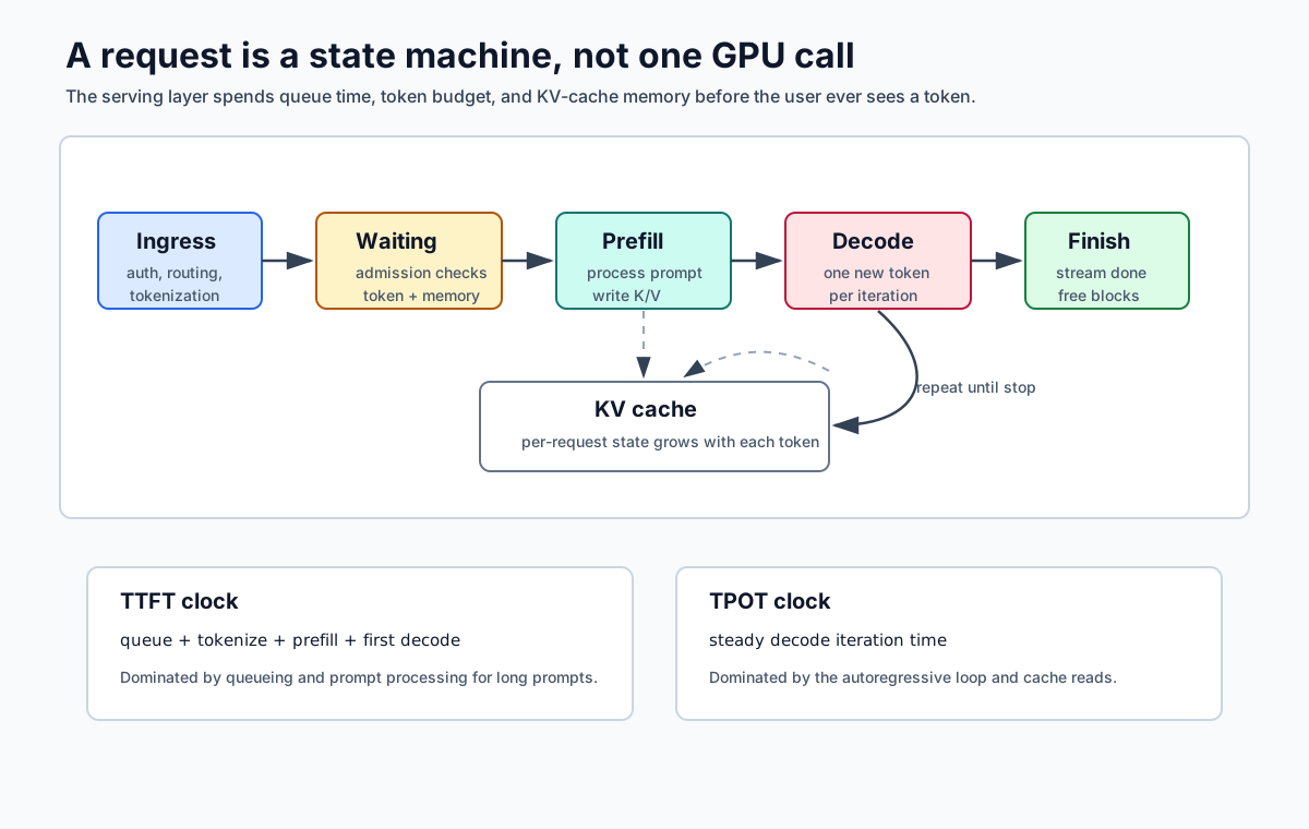
At minimum, a serving engine has to manage these states:
WAITING_PREFILL
  -> PREFILLING
  -> WAITING_DECODE
  -> DECODING
  -> FINISHED | CANCELLED | PREEMPTED
The important detail is that PREFILLING and DECODING are not the same workload.
During prefill, the server processes the prompt tokens that already exist. It computes the attention state for those tokens and writes each layer’s keys and values into the KV cache. Long prompts make prefill expensive. A 40,000-token prompt is not “just one request” from the GPU’s point of view; it is a large block of context work that may interfere with many users already waiting for their next streamed token.
During decode, each active sequence produces one new token per model iteration. The server reads the request’s existing KV cache, computes logits for the next token, samples or selects that token, appends the token’s new KV entries, streams the token, and repeats.
That gives us the first useful latency decomposition:
TTFT ~= queue_time
      + tokenization_time
      + prefill_schedule_delay
      + prefill_execution_time
      + first_decode_iteration

E2E_latency ~= TTFT + (output_tokens - 1) * TPOTTTFT, time to first token, is what tells a user “the system is alive.” It is dominated by queueing and prefill for long prompts.
TPOT, time per output token, is what makes streaming feel smooth or broken. It is dominated by the steady decode loop.
Optimizing only blended tokens/sec can hide damage to both. A throughput improvement that increases TTFT for interactive users may be a product regression. A low TTFT system that produces unstable inter-token gaps can still feel bad. A serious inference system tracks both clocks.
Prefill and decode live on different parts of the roofline
The reason prefill and decode interfere is not just that one is “long” and the other is “short.” They stress the GPU differently.
In prefill, the model has many prompt tokens available at once. Matrix multiplications are larger. Attention over the prompt is expensive, but there is enough parallel work to keep the GPU busy. FlashAttention’s core insight is relevant here: standard attention wastes time moving large intermediate tensors between GPU high-bandwidth memory and on-chip SRAM. FlashAttention is IO-aware; it tiles attention so it computes exact attention with fewer HBM reads and writes than the naive approach.
Decode is different. For one sequence, each step has exactly one new query token. That new token attends over the old keys and values. The work per sequence is small, and the historical KV state grows with context length. In the multi-query attention paper, Noam Shazeer describes incremental inference as slow partly because of the memory-bandwidth cost of repeatedly loading the keys and values. That is the decode pain in one sentence.
Batching helps decode because the model weights can be reused across many active sequences in the same iteration. But batching is not free. More active sequences mean more KV cache residency, more scheduler complexity, and often higher queuing latency.
The useful simplification is:
Prefill: many known tokens -> larger compute tiles
Decode:  one new token  -> repeated reads of old state
For a single long-context sequence, one decode step may touch KV state proportional to the entire active context:
decode_kv_read_per_new_token ~=
  layers * 2 * kv_heads * context_tokens * head_dim * bytes_per_value
The exact traffic depends on kernels, tensor parallelism, locality, quantization, and cache layout. But the shape is the point. Decode gets more memory-hungry as context grows, even though it emits only one token.
That is the first real inference trade-off:
More batching -> better GPU utilization and throughput
More batching -> more waiting, more KV memory, worse tail risk
The job is not to maximize batch size. The job is to admit the right work at the right time.
The KV cache is the second model
For each token, each transformer layer stores two tensors for future attention: a key and a value. This is the KV cache.
The basic formula is:
kv_cache_bytes_per_sequence =
  tokens
  * layers
  * 2                 # key + value
  * kv_heads
  * head_dim
  * bytes_per_value
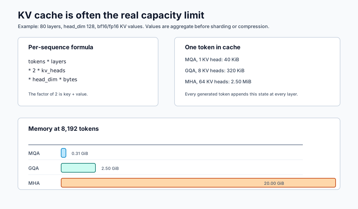
For a Llama-like 70B-class GQA shape with 80 layers, 8 KV heads, head dimension 128, and bf16/fp16 KV values:
bytes_per_token = 80 * 2 * 8 * 128 * 2
                = 327,680 bytes
                = 320 KiB per token
That sounds manageable until you multiply by context and concurrency.
| Context per sequence | KV cache per sequence | 32 active sequences |
|---|---|---|
| 8,192 tokens | 2.50 GiB | 80.00 GiB |
| 16,384 tokens | 5.00 GiB | 160.00 GiB |
| 131,072 tokens | 40.00 GiB | 1.25 TiB |
Those are aggregate KV numbers before implementation-specific tensor-parallel sharding, compression, offload, or eviction. The point is not the exact deployment number. The point is the scale: the cache is a first-class capacity constraint.
The same table also explains why decode latency gets harder at long context. In the 8,192-token row, a single generated token for one sequence can require reading on the order of 2.50 GiB of KV state across the model. With 32 active sequences at that context length, the aggregate KV state participating in a decode iteration is on the order of 80 GiB. The implementation may shard and optimize that movement, but the serving system still has to schedule around it.
Here is a concrete capacity envelope. Suppose a 70B-class model uses bf16 weights: roughly 140 GB, or about 130 GiB, before runtime overheads. With tensor parallelism across 4 GPUs, the weights are roughly 32.5 GiB per GPU if evenly sharded. On an 80 GB GPU, that may leave something like 35-40 GiB per GPU for KV cache after workspaces, runtime overhead, fragmentation, and safety margin.
If KV cache is also sharded across those 4 GPUs, the 8,192-token GQA example consumes about 0.625 GiB per GPU per active sequence:
2.50 GiB aggregate KV / 4-way tensor parallel ~= 0.625 GiB per GPUA 35 GiB per-GPU KV budget would fit at most about 56 such sequences before accounting for allocator slack, output growth, prefix-cache retention, or preemption policy. At 16,384 tokens, that drops to about 28 sequences. This is why admission control cannot be an afterthought. The scheduler is not only asking “is there room for this prompt?” It is asking “is there room for this request’s future?”
This is why multi-query attention and grouped-query attention show up in inference conversations so often.
With standard multi-head attention, the number of KV heads usually matches the number of query heads. If the same 70B-class shape used 64 KV heads instead of 8, the KV cache would be 8x larger:
| Attention layout | KV heads | KV per token | KV at 8,192 tokens |
|---|---|---|---|
| Multi-head | 64 | 2.50 MiB | 20.00 GiB |
| Grouped-query | 8 | 320 KiB | 2.50 GiB |
| Multi-query | 1 | 40 KiB | 320 MiB |
Multi-query attention shares one set of keys and values across query heads, reducing KV memory and bandwidth in incremental decoding. Grouped-query attention is the middle ground: more than one KV head, fewer than the number of query heads. The GQA paper frames this explicitly as a way to approach multi-head quality while retaining much of the speed benefit of multi-query attention.
This is a model architecture decision, not only a serving decision. You cannot retrofit it casually without quality work. But from the serving side, the implication is clear: KV heads are an inference budget.
Continuous batching is admission control
Classic batching groups requests, runs the batch, and returns results. That falls apart for generative models because request lengths are wildly different.
One request may finish after 12 generated tokens. Another may generate 2,000. If the server waits for the whole batch to finish, short requests are trapped behind long ones. If the server refuses new work until a batch drains, the GPU sees gaps even while users are queued.
Orca introduced the right mental model: schedule at the granularity of a model iteration rather than a whole request. Every decode iteration becomes a chance to:
- remove finished requests
- admit new requests
- choose which prefills to run
- choose which decodes get their next token
- respect memory and token budgets
NVIDIA TensorRT-LLM calls the same broad idea in-flight batching, also known as continuous batching or iteration-level batching. Its public docs also call out two knobs that matter more than they first appear: max_batch_size and max_num_tokens. The second one is crucial because a batch is not just “number of requests.” A batch is also a token budget.
Here is the shape of a simple decode-first scheduler:
while server_is_running:
    batch = Batch(token_budget=max_num_batched_tokens)

    # 1. Keep streams moving.
    for req in running_decode_queue:
        if batch.has_budget(1) and kv_cache.can_append(req, tokens=1):
            batch.add_decode(req, tokens=1)

    # 2. Admit prompt work without letting it swallow the iteration.
    while batch.has_budget(min_prefill_chunk):
        req = waiting_prefill_queue.peek()
        if req is None:
            break

        chunk = min(req.remaining_prompt_tokens,
                    prefill_chunk_size,
                    batch.remaining_token_budget)

        if not kv_cache.can_reserve(req, tokens=chunk):
            break

        batch.add_prefill(req, tokens=chunk)
        waiting_prefill_queue.advance_if_done(req)

    outputs = model.forward(batch)
    kv_cache.commit(outputs.kv_writes)
    stream_new_tokens(outputs.decode_tokens)
    free_finished_requests()
Real engines are more complex. They handle priorities, preemption, cancellation, prefix hits, tensor parallelism, CUDA graph capture constraints, LoRA adapters, tool-calling constraints, and fairness. But this skeleton shows the core: the scheduler is spending a scarce token budget and a scarce KV-cache budget every iteration.
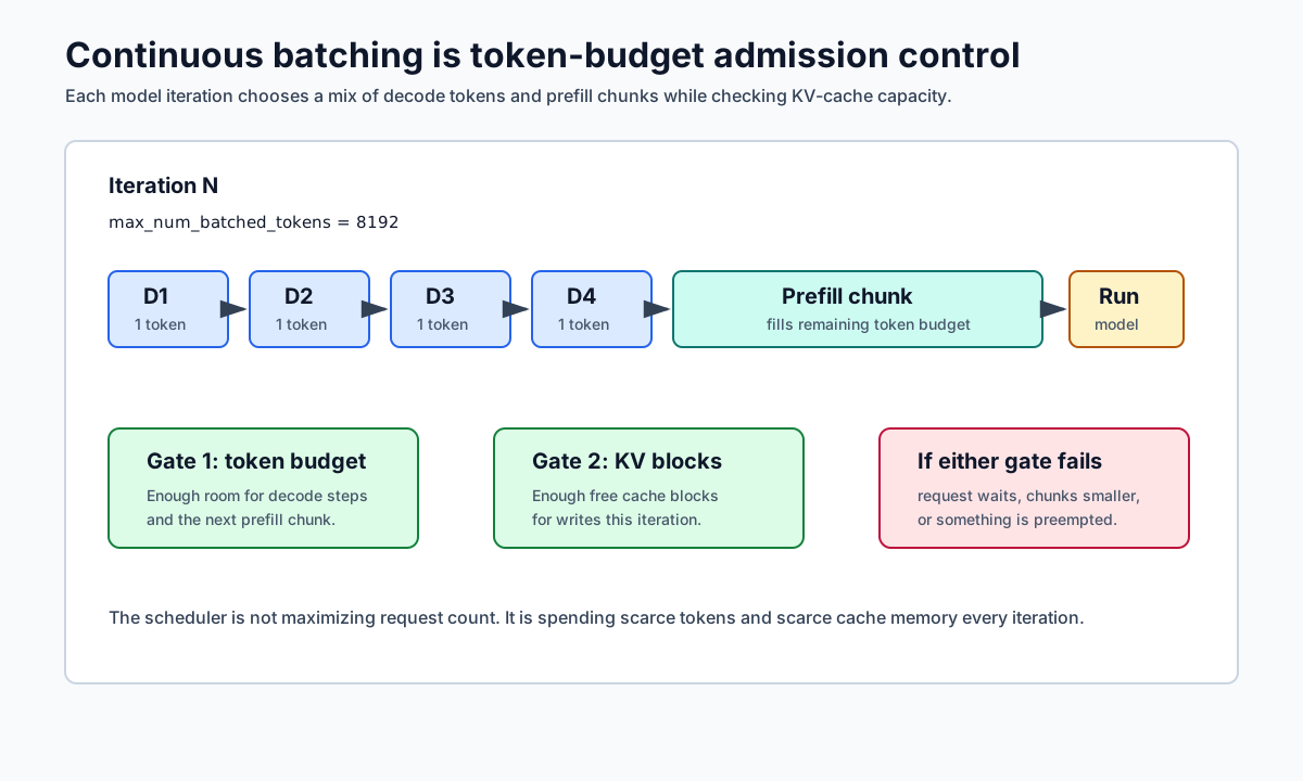
This is also why a single “GPU utilization” number is not enough. A server can show high GPU utilization while interactive decode streams are waiting behind long prefills. A server can show moderate utilization while delivering excellent TTFT and TPOT for the product’s actual SLO. Good inference engineering is about goodput: useful work completed within the latency target.
The scheduler invariants I would want are boring but important:
- An admitted request has a clear KV-cache plan: reserve, grow on demand, preempt, or reject.
- Decode streams have a bounded maximum skip count so prefill cannot silently break streaming.
- Prefill has a chunk policy tied to latency SLOs, not just a global constant.
- Prefix-cache hits do not bypass tenant isolation, model versioning, or prompt-template versioning.
- Every speculative path has a kill switch and route-level eligibility rules.
Those invariants matter more than the exact data structure. They are what keep a clever scheduler from becoming an incident generator.
Admission policy is where product priorities become real. Interactive chat may get decode-first scheduling because streaming smoothness matters. Agent runs may tolerate longer TTFT if they are tool-heavy and less human-visible. Batch summarization or eval traffic can fill slack but should not steal token budget from live sessions. A cancelled stream should release KV blocks promptly, because a disconnected user holding cache is indistinguishable from a memory leak.
Chunked prefill reduces decode interference
A long prefill can monopolize an iteration.
Suppose the engine has a max_num_batched_tokens budget of 8,192. If a new request arrives with a 32,000-token prompt, a naive scheduler either rejects it for the current iteration or schedules a giant prefill that blocks decode progress for requests already streaming.
Chunked prefill splits that prompt into smaller pieces. Instead of asking “can I run the whole prompt now?”, the scheduler asks “can I run the next chunk now and still keep decode moving?”
The SARATHI paper describes this as chunked prefills plus decode-maximal batching: use a prefill chunk to saturate compute, then let decode requests piggyback in the remaining batch structure. TensorRT-LLM’s docs describe the same mechanical idea as chunked context: split context into chunks so context work can be batched with generation work.
The production trade-off follows from that mechanism. Chunking can improve interference behavior for mixed prefill/decode traffic, but it may also delay completion of a request that could have run its full prefill immediately on an otherwise idle system.
That is exactly the kind of trade-off an inference engineer should be comfortable with. Chunking is not “faster” in a vacuum. It changes interference.
The question is:
Do I want one full-prefill request to finish immediately,
or do I want stable decode progress and better tail behavior?
For an interactive product, the second answer is often the right one.
Paged KV cache is virtual memory for attention state
If KV cache is the second model, then the cache manager is the operating system.
A simplifying baseline KV layout preallocates a contiguous cache region for every request up to the maximum sequence length:
[max_sequences, max_seq_len, layers, 2, kv_heads, head_dim]That is simple and wasteful. Most requests do not use the maximum length. Some finish early. Some share prefixes. Some are cancelled. Some grow for thousands of decode iterations. Static reservation turns average-case traffic into peak-case memory pressure.
PagedAttention, introduced with vLLM, attacks this by splitting KV cache into fixed-size blocks. Each request has a logical sequence of token positions. A block table maps those logical positions to physical KV blocks.
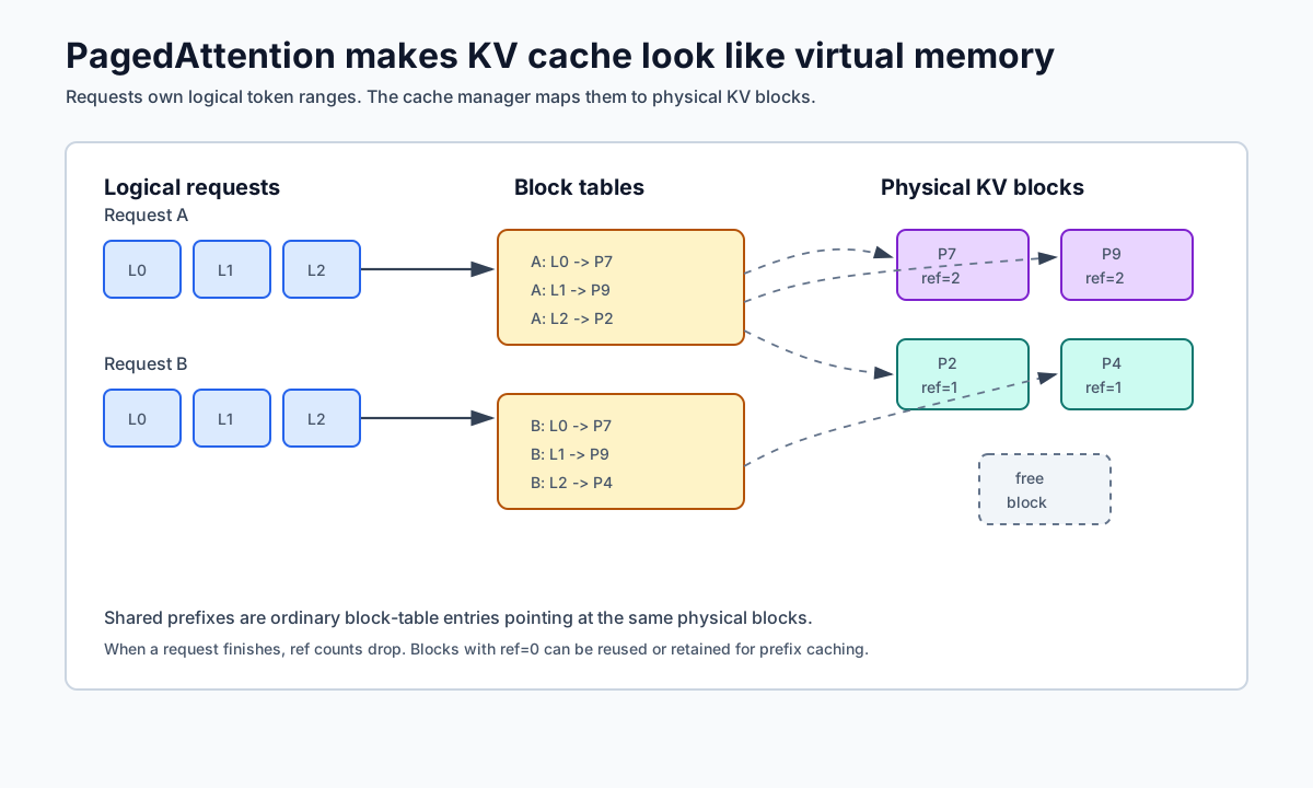
This unlocks three practical behaviors:
Allocation on demand. A request receives more blocks as it grows. It does not reserve the maximum context length on admission.
Low internal waste. The only unavoidable slack is usually in the final partially filled block, rather than across an entire max-length reservation.
Sharing. If two requests share a prefix, their logical block tables can point at the same physical blocks with reference counts.
The trade-off is indirection. Attention kernels need to understand block tables. The scheduler needs to coordinate allocation and eviction. Prefix reuse requires correct hashing and isolation. But the payoff is large because KV cache is often what limits batch size.
The vLLM paper makes the operational point directly: inefficient KV-cache management wastes memory through fragmentation and redundant duplication, limiting batching. Once you accept that, paging stops looking like clever infrastructure and starts looking like the natural shape of the problem.
Prefix caching is routing, not just caching
Prompt caching is often described as a cost feature. Underneath, it is a serving feature.
If two requests share a long prefix - system instructions, tool schemas, few-shot examples, retrieved documents, or conversation history - a self-hosted engine can literally reuse computed attention state for that prefix. For hosted APIs, the public documentation exposes the behavior rather than the full implementation. OpenAI’s prompt caching docs describe routing requests to servers that recently processed the same prompt, and its extended caching docs refer to key/value tensors. That is enough to reason about the system without pretending to know private internals.
But cache reuse only works when the request lands where the cache exists, and only when the reusable part is actually identical.
OpenAI’s prompt caching docs describe exact prefix matching, automatic activation for prompts of at least 1,024 tokens, cached_tokens in usage details, and routing influenced by the prompt prefix and optional prompt_cache_key. Anthropic’s docs expose cache_creation_input_tokens and cache_read_input_tokens, support cache breakpoints, and recommend putting stable reusable content at the beginning of the prompt.
Those API details reveal the serving mechanics:
stable prefix -> routing key -> cache lookup -> reused KV tensors
variable suffix -> ordinary prefill/decode work
The prompt layout matters. This is bad for caching:
timestamp
request id
user-specific metadata
tool definitions
system instructions
long shared document
actual user question
This is better:
system instructions
tool definitions
long shared document
few-shot examples
user-specific metadata
timestamp
actual user question
The first layout poisons the prefix with variables. The second keeps the expensive reusable material stable.
There is also a security dimension. Prefix-cache hits can create timing differences. Public systems document isolation boundaries: OpenAI says prompt caches are not shared between organizations; Anthropic documents workspace-level and organization-level isolation depending on platform; vLLM supports a cache_salt to isolate prefix-cache reuse for shared environments.
That makes prefix caching a routing and isolation problem, not only an optimization.
Disaggregated serving separates the two clocks
Once the prefill/decode split is clear, a bigger architecture question appears:
Should prefill and decode run on the same GPU pool?Colocating them is simpler. The prefill phase writes KV cache locally, and the decode phase consumes it locally. No KV transfer is needed.
But colocating them also couples two different workloads. A long prefill can interfere with decode latency. Decode-heavy traffic can leave prefill capacity under-shaped. The parallelism strategy that works well for prefill may not be ideal for decode.
DistServe frames this as goodput optimization under TTFT and TPOT constraints: assign prefill and decode computation to different GPUs, co-optimize resource allocation and parallelism per phase, and place phases with network bandwidth in mind. NVIDIA Dynamo’s public docs describe the same broad design in production terms: prefill workers compute KV cache, transfer it, and decode workers generate tokens.
Disaggregation introduces a new cost:
prefill GPU -> KV transfer -> decode GPUThat transfer can be enormous for long prompts. So disaggregation is not automatically better. It wins when reduced interference and better phase-specific scaling outweigh KV-transfer cost.
This is the mature inference answer to many architecture questions: “it depends” is not a dodge if you can name the dependency.
For disaggregated serving, the dependencies are:
- prompt length distribution
- output length distribution
- TTFT and TPOT SLOs
- network bandwidth between workers
- tensor-parallel strategy per phase
- KV-cache transfer format
- cache locality and prefix reuse
- failure behavior when prefill succeeds but decode placement changes
That is the kind of surface area where inference engineering starts looking like distributed systems again.
Speculative decoding attacks the serial dependency
The decode loop has an unavoidable dependency: token t + 1 depends on token t.
Speculative decoding tries to reduce the wall-clock cost of that dependency. A faster draft model proposes several future tokens. The larger target model verifies them in parallel. The original speculative decoding paper shows how to do this without changing the target model’s output distribution under the algorithm’s sampling procedure.
The simplest mental model:
1. Draft model proposes:  d1, d2, d3, d4
2. Target model evaluates those positions in one pass.
3. Accept the longest valid prefix.
4. If a token is rejected, sample from the corrected target distribution.
5. Repeat.
The serving question is whether the target model gets enough accepted tokens per verification pass to justify the draft work.
This is where implementation details matter. Exact speculative sampling, greedy verification, n-gram speculation, tree-based proposals, Medusa-style heads, and model-native prediction heads all live in the same family of ideas, but they do not have identical correctness or performance properties. Acceptance rate depends on temperature, task type, tokenizer alignment, structured-output constraints, and how often the target model disagrees with the proposer.
Useful metrics:
- draft tokens proposed per step
- accepted tokens per target pass
- rejection position distribution
- draft model latency
- target verification latency
- wasted draft work
- interaction with continuous batching
Speculation can reduce TPOT. It can also waste compute if the draft model is poorly matched, if prompts are distribution-shifted, if structured decoding rejects many proposals, or if the serving engine is already throughput-saturated and would rather use that capacity for ordinary batches.
It is not a magic switch. It is a bet on acceptance rate and scheduler fit.
The hidden constraints: shapes, graphs, and kernels
At the kernel layer, inference engines fight a second battle: the GPU likes stable shapes, while user traffic is dynamic.
Static shapes are friendly to compilation and CUDA graph capture. Dynamic traffic produces variable batch sizes, variable sequence lengths, variable prefix-cache hits, variable decode counts, and variable adapter/tool constraints.
That tension shows up everywhere:
- Static KV caches can be friendly to JIT or graph capture, but reserve memory.
- Dynamic KV caches save memory, but complicate compilation and indexing.
- Paged KV cache improves utilization, but attention kernels need page-table aware memory access.
- Prefix caching saves prefill work, but creates routing and eviction complexity.
- Chunked prefill reduces interference, but changes per-request TTFT distribution.
Here is the concrete version of that tension. CUDA graphs prefer a stable captured shape. Continuous batching changes the active request set every iteration. Engines often respond by bucketing shapes, capping token budgets, padding or packing into known profiles, and separating a graph-captured decode path from a more dynamic prefill path. Each choice spends a different budget: padding spends compute, many profiles spend build and memory overhead, dynamic paths spend launch overhead, and strict bucketing can spend latency.
Libraries like FlashInfer are interesting because they sit at this boundary: kernel-level attention performance, heterogeneous KV-cache formats, dynamic request scheduling, and CUDA graph compatibility. That is the real shape of modern inference work. It is not one trick. It is a negotiation between workload variability and hardware preferences.
How I would debug an inference service
If an inference service is slow, I would not start by swapping engines. I would first turn the incident into one of four shapes.
| Symptom | First question | Common suspect |
|---|---|---|
| High TTFT, normal TPOT | Are requests waiting before first decode? | queueing, long prefill, cold prefix cache |
| Normal TTFT, high TPOT | Are decode iterations stretched? | KV bandwidth, batch shape, kernel path, speculation misses |
| High TTFT and high TPOT | Is the replica overloaded or memory-bound? | admission, KV pressure, bad routing, noisy tenant |
| Good latency, bad cost | Are we doing redundant work? | prefix-cache misses, poor batching, overprovisioning |
That classification matters because each failure asks for a different experiment. If TTFT is broken, I care about queueing, prefill, and prefix reuse. If TPOT is broken, I care about decode batch shape, KV reads, kernel efficiency, and inter-token gaps. If both are broken, I suspect admission control or memory pressure before I suspect one kernel.
Now make it concrete.
Imagine a deployment lands and the dashboard shows this:
p95 TTFT:  0.9s -> 3.8s
p95 TPOT:  unchanged
error rate: unchanged
GPU utilization: slightly higher
The first inference is that the steady decode loop is probably not the primary issue. Users are waiting longer for the first token, but once generation starts, streaming is healthy. That pushes the investigation toward routing, queueing, prefix lookup, prefill, and KV admission.
The trace I want for every request is:
request_received
  -> routed_to_replica
  -> prefix_cache_lookup_done
  -> admitted_for_prefill
  -> prefill_started
  -> prefill_finished
  -> first_decode_started
  -> first_token_streamed
  -> decode_iteration[n]
  -> final_token_streamed
  -> kv_blocks_released
Then I compare the broken cohort with a healthy one. In this hypothetical incident, the pattern is:
| Signal | Healthy template | Regressed template |
|---|---|---|
| queue time | unchanged | unchanged |
| prefill execution | normal | 3x higher |
| prefix-cache hit rate | 71% | 9% |
| cached/read tokens | high | near zero |
| active decode batch | unchanged | unchanged |
| TPOT | unchanged | unchanged |
| KV admission failures | rare | rare |
That narrows the problem. The scheduler is not obviously starving decode. The KV cache is not blocking admission. The decode path is healthy. The regressed template is simply doing much more prefill work than before.
Next I would diff the tokenized prefixes, not the raw strings. Exact-prefix caching is token-based behavior; invisible whitespace, JSON ordering, timestamp placement, and template version strings can all matter.
The bug might look like this:
Expected stable prefix:
  system instructions
  tool schema
  policy document
  examples
  request metadata
  user question

Actual prefix after deploy:
  system instructions
  request_id
  trace timestamp
  tool schema
  policy document
  examples
  user question
The volatile fields moved before the expensive stable content. Every request now has a different prefix before it reaches the tool schema, so the cache lookup misses. The model is not slower. The prompt layout broke locality.
The fix is not “buy more GPUs.” The fix is:
- move volatile fields after stable reusable content
- include prompt template version in the cache/routing key
- keep tenant and isolation salt unchanged
- replay a production-like trace before and after
- verify TTFT without damaging TPOT
The proof should be visible in a small before/after table:
| Metric | Before fix | After fix |
|---|---|---|
| prefix-cache hit rate | 9% | back near previous baseline |
| cached/read tokens | near zero | recovered |
| prefill tokens executed | high | lower for repeated prefixes |
| p95 TTFT | elevated | recovered |
| p95 TPOT | unchanged | unchanged |
| KV evictions | unchanged | unchanged |
That is the shape of a good inference diagnosis: a user-visible symptom, a phase-level split, a state/locality explanation, and proof that the fix repaired the mechanism without moving pain somewhere else.
Different symptoms take different branches. If TPOT regressed while TTFT stayed stable, I would inspect active decode batch size, inter-token gap, attention backend, KV-read pressure, CUDA graph hit rate, collective communication, and speculative acceptance. If both TTFT and TPOT regressed, I would look for admission pressure, KV exhaustion, noisy tenants, or routing imbalance. If latency stayed good but cost rose, I would hunt redundant prefill, cache misses, over-batching, and overprovisioned replicas.
The goal is to end with an incident sentence that names the mechanism:
Bad:  GPU is slow.
Good: p95 TTFT regressed because template v17 moved volatile metadata
      before the stable tool schema, dropping prefix-cache hits and pushing
      more long prefills into the decode window while TPOT stayed healthy.
That is the difference between observing a slow model and debugging an inference system.
Failure modes I would look for first
The prompt template breaks its own cache. A timestamp, request id, user name, or volatile retrieval snippet appears before the stable tool schema. Exact-prefix caching loses.
The scheduler optimizes throughput into bad UX. Large batches look good in aggregate tokens/sec but damage p95 TTFT or TPOT.
The KV cache is treated as an implementation detail. Admission succeeds because weights fit, then decode stalls or preempts because per-request KV growth was underestimated.
Chunked prefill is tuned like a constant. A chunk size that works for short-chat traffic may be wrong for long-document summarization or agent traces.
Disaggregation ignores transfer. Separating prefill and decode helps only if KV movement, placement, and failure behavior are part of the design.
Speculation is benchmarked in isolation. Draft acceptance looks good offline, then production batching pressure makes the extra draft work less attractive.
Quantization is measured without quality gates. Weight quantization, activation quantization, and KV-cache quantization have different risk profiles. Speed without evals is not an engineering result.
What strong inference engineering looks like
Strong inference engineering is the ability to hold three layers in your head at the same time.
At the model layer, you understand autoregressive dependencies, attention variants, KV heads, context length, sampling, and quality risk.
At the kernel layer, you understand memory bandwidth, HBM traffic, tensor shapes, attention kernels, graph capture, quantization formats, and communication collectives.
At the systems layer, you understand admission control, continuous batching, cache allocation, prefix-aware routing, tenant isolation, disaggregated placement, SLOs, and cost per useful token.
The best work happens where those layers meet.
PagedAttention is not just an attention trick; it is memory management for a dynamic serving workload. Chunked prefill is not just prompt splitting; it is interference control. Prompt caching is not just a discount; it is prefix-aware routing and KV reuse. Speculative decoding is not just a smaller model; it is a scheduler-level bet on accepted tokens per verification pass.
That is why I like this problem. LLM inference is where machine learning becomes operating systems, distributed systems, and performance engineering all at once.
The model answers the user. The serving system decides whether it answers quickly enough to matter.
Further Reading
- Attention Is All You Need
- FlashAttention: Fast and Memory-Efficient Exact Attention with IO-Awareness
- Fast Transformer Decoding: One Write-Head is All You Need
- GQA: Training Generalized Multi-Query Transformer Models from Multi-Head Checkpoints
- Orca: A Distributed Serving System for Transformer-Based Generative Models
- Efficient Memory Management for Large Language Model Serving with PagedAttention
- SARATHI: Efficient LLM Inference by Piggybacking Decodes with Chunked Prefills
- DistServe: Disaggregating Prefill and Decoding for Goodput-optimized LLM Serving
- TensorRT-LLM: Paged Attention, In-Flight Batching, and Request Scheduling
- NVIDIA Dynamo: Disaggregated Serving
- vLLM Automatic Prefix Caching Design
- Hugging Face Transformers: KV Cache Strategies
- Fast Inference from Transformers via Speculative Decoding
- FlashInfer: Efficient and Customizable Attention Engine for LLM Inference Serving
- OpenAI Prompt Caching
- Anthropic Prompt Caching